Coefficient paths and cross-validation curves

This example demonstrates some of the properties of the FRR approach and compares it to the use of standard ridge regression (RR) on the diabetes dataset that is included in sckit-learn.

In standard ridge regression, it is common to select alpha by testing a range of log-spaced values between very minimal regularization and very strong regularization. In fractional ridge regression, we instead select a set of frac values that represent the desired reduction in the L2-norm of the coefficients.

Imports:

import numpy as np
import matplotlib.pyplot as plt

This is the Fracridge sklearn-style estimator:

from fracridge import FracRidgeRegressor

from sklearn import datasets
from sklearn.linear_model import Ridge
from sklearn.model_selection import cross_val_predict
from sklearn.metrics import r2_score

Get example data from scikit learn:

X, y = datasets.load_diabetes(return_X_y=True)

Values of alpha for the standard approach are set to be 20 values That are log-spaced from a very small value to a very large value:

n_alphas = 20
rr_alphas = np.logspace(-10, 10, n_alphas)
rr_coefs = []
rr_coefs = np.zeros((X.shape[-1], n_alphas))
rr_pred = np.zeros((y.shape[-1], n_alphas))

We calculate the fit and cross-validated prediction for each value of alpha:

for aa in range(len(rr_alphas)):
    RR = Ridge(alpha=rr_alphas[aa], fit_intercept=True)
    RR.fit(X, y)
    rr_coefs[:, aa] = RR.coef_
    rr_pred[:, aa] = cross_val_predict(RR, X, y)

In contrast, FRR takes as inputs fractions, rather than arbitrarily-chosen values of alpha. The alphas that are generated are selected to produce solutions whos fractional L2-norm relative to the L2-norm of the unregularized solution are these values. Here too, cross-validated predictions are generated:

fracs = np.linspace(0, 1, n_alphas)
FR = FracRidgeRegressor(fracs=fracs, fit_intercept=True)
FR.fit(X, y)
fr_pred = cross_val_predict(FR, X, y)

We plot the results. First, the FRR coefficients as a function of requested fractions and then the RR coefficient as a function of the requested log-spaced alpha:

fig, ax = plt.subplots(1, 2)
ax[0].plot(fracs, FR.coef_.T)
ylims = ax[0].get_ylim()
ax[0].vlines(fracs, ylims[0], ylims[1], linewidth=0.5, color='gray')
ax[0].set_ylim(*ylims)
ax[1].plot(np.log(rr_alphas[::-1]), rr_coefs.T)
ylims = ax[1].get_ylim()
ax[1].vlines(np.log(rr_alphas[::-1]), ylims[0], ylims[1], linewidth=0.5,
             color='gray')
ax[1].set_ylim(*ylims)

Out:

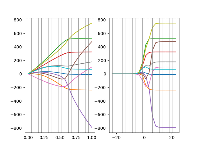
(-869.3480959251679, 828.4461624666238)

In a second plot, we compare the cross-validated predictions with the original data. This is appropriate as each prediction was generated in a sample that did not include that observation.

test_y = np.tile(y, (fr_pred.shape[-1], 1)).T

rr_r2 = r2_score(test_y, rr_pred, multioutput="raw_values")
fr_r2 = r2_score(test_y, fr_pred, multioutput="raw_values")

fig, ax = plt.subplots(1, 2, sharey=True)
ax[0].plot(fracs, fr_r2, 'o-')
ylims = ax[0].get_ylim()
ax[0].vlines(fracs, ylims[0], ylims[1], linewidth=0.5, color='gray')
ax[0].set_ylim(*ylims)

ax[1].plot(np.log(rr_alphas[::-1]), rr_r2, 'o-')
ylims = ax[1].get_ylim()
ax[1].vlines(np.log(rr_alphas[::-1]), ylims[0], ylims[1], linewidth=0.5,
             color='gray')
ax[1].set_ylim(*ylims)


plt.show()